Scaling or not?

Introduction
Scaling in short
Best Practices
Conclusion

Introduction

It is becoming easier and easier to run complex parallel programs on the cluster. This is of course a great potential advantage to researchers and student, that can have more results, and in less time. This also means that an inexperienced user can easily run massively parallel programs. But sometimes the performance is not the one one expects.

One of the main reason is due to the expectations related to parallelization. One could expect naively that “if my program needs 24 hours to complete on one processor, then, if I use 24 processors, it will take 1 hour!”. This often leads the users to use the maximum number of processors they are allowed to use on the cluster, hoping to have their results faster.
This sentence is not wrong, in principle. This kind of behaviour (linear scaling) is possible, for the so-called embarrassingly parallel programs, i.e. programs in which each processor executes a part of code that is completely independent from the other. And it also requires that each of the independent parts takes almost exactly the same time. In some special condition, even a better scaling (superlinear) can be achieved. But this is more the exception, than the rule.

We do not go deep into these problem, but instead give some practical hints.

Scaling in short

Running a parallel program, one aims at improving the performance with respect to a serial program. Let us focus here on the execution time. We therefore measure the performance in terms of speedup.
The speedup is exactly what one should expect: it is defined as the ratio of the execution time of a program run on 1 processor t(1), to execution time of a program run on N processor t(N):

Sp(N)=t(1)/t(N)

In the best case scenario (if we exclude the superlinear scaling), this speedup can be estimated via the Amdahl’s law.
Let us assume that a program is made of two parts: one that in intrinsically serial, and one that is parallelizable. The total execution time of the program on a single processor, will then be

t(1) = t_S+ t_P(1)

We can define the Serial fraction S=t_S/t(1), and the Parallel fraction P=t_P(1)/t(1). In this way,

t(1)=S*t(1)+P*t(1)

t(1)=(1-P)*t(1) + P*t(1)

If one now runs the same program on N processors, the time will be:

t(N)=t_S + t_P(N).

But t_S will be exactly the same, since it is serial. And in the best case scenario, t_P(N)=t(1)/N.
So

 t(N) = (1-P)*t(1) + P/N*t(1)

We can therefore estimate the speedup:

Sp(N)=t(1)/t(N)=t(1)/[(1-P)*t(1) + P/N*t(1)] = 1/[(1-P) + P/N]

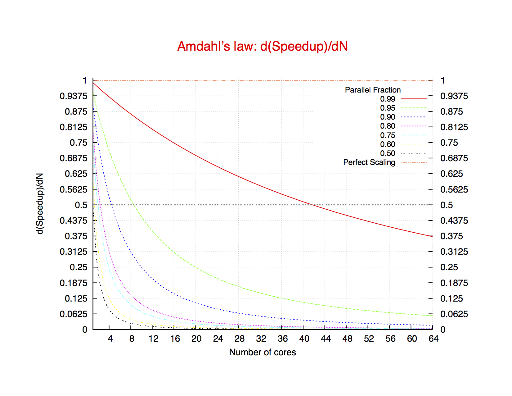
Fig. 2: Theoretical Derivative of the Speedup, according to Amdahl’s law, for different values of the parallel fraction.

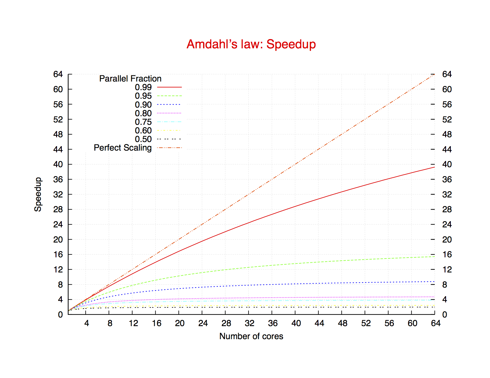
Fig. 1: Theoretical speedup according to Amdahl’s law for different values of the parallel fraction.

Comments:

This shows two things:

There is a maximum speedup, that is 1/(1-P). This is trivial: even using infinitely many processors, the program will not run faster than it serial part. Notice for example that when P=0.9, that is the program spends 90% of the time in the parallelizable fraction, the maximum speedup is 10. (Fig. 1)
The speedup curve becomes flatter, increasing the number of processors used. This means that the speedup one gets adding one processors becomes smaller and smaller. At a certain point, it doesn’t pay off any more (Fig. 2)
A rough approximation is that if the speedup with N cores is S(N), then the speedup with N+1 is
```
S(N) + d(speedup(N))/dN * 1
```
In case of perfect speedup, d(speedup(N))/dN is identically 1, so each new core counts as 1. As can be seen from the formula and the picture on the right, adding 1 cores gives less than an extra 0.5 of speedup, even with a 99% parallel code, above 40 cores. For a 95% parallel core, this happens at a value as low as 9.

The conclusion is that it is not always worth to use many cores in a program unless it scales very very well. And this MUST be tested.

Note:
All these considerations holds only for the speedup. If the purpose of adding cores is not to make the program faster, but to be able to do more work have a look at see Gustafson’s law.

Best Practices

The discussion of the previous section can be instructive, but how to proceed in reality? We can try to give some common sense instructions, here.

1. How do I know how much is the parallel fraction of my program?
  It is alway better not try to guess, and instead to “measure” it. The Amdahl’s law is oversimplified, and describes a kind of best case scenario. But in a complex program, there are many things that can affect the performance. So it is always better to make some tests.
  - Rough estimate: Run a your program with N cores. Estimate
```
RSp=(Total cputime)/(user Time).
```
  This is a very rough estimate of your speedup. Then a rough estimate of your parallel fraction is:
```
P_Frac=(1-RSp)*N/[RSp*(1-N)]
```
  - Accurate estimate: Define a test case (long enough so that the effect of system startup and cleanup are not relevant even when using many cores), and run the same test case, changing the number of cores.
    In this way you can have some points to make the a graph like the one of Fig.1. From that, you can fit the parallel fraction P_m (where the “m: stands for “measured”, and so get a number. This will tell you that your program scales as an ideal Amdal’s law program with a parallel fraction of P_m. Then based on this P_m value, you can estimate the “ideal” number of cores to use.
2. Which is the ideal number of cores?
  There is not a unique answer. If you have resources to waste, you don’t have any problem. But this is usually not what happens in a cluster. So, let us assume that you have 80 cores available, and you have
  Number of cores | Parallel Fraction: 0.90 | Parallel Fraction: 0.99
  ——————————————————————————————
  80      |          2h 40 min         |                     0h 32 min
  40                          |                      2h 57 min      |                     0h 50 min
  20                          |                      3h 29 min         |                     1h 26 min
  As can be seen, there is almost no convenience in using 80 cores instead of 40, for P=0.90. And using half of the available cores, means that one can run two models simultaneously, and get the results of two runs in almost the same time…

Conclusion:

Spend some time in benchmarking your code if you do not want to waste time and resources later